Resolution, Accuracy, and Precision of Encoders
When you’re choosing an encoder for a motion control system, you’ll be faced with numerous technical terms. The amount of data available can be overwhelming. Which critical terms should you focus on first, and which can be deferred?
This article looks at three important concepts that deserve your attention: resolution, accuracy and precision.
At first glance, it may seem that all three mean roughly the same thing. You may wonder if they’re interchangeable; indeed, many people speak of them as if they are. After all, if an encoder has high resolution, doesn’t that mean it’s accurate? And if it’s accurate, then it has to be precise, right? (Please note: the answer to these last two questions is a firm no.)
In fact, the terms are independent of each other. Each refers to a specific encoder characteristic, and they are not interchangeable. To clear up any confusion, we’ll first explain what resolution means for incremental encoders, then note any differences for linear and absolute encoders. We’ll move on to accuracy, and finish with precision. Along the way, we’ll give tips on how to use knowledge about each term to make the best encoder selection, and how to calibrate a system once the encoder is in place.
RESOLUTION
In math, science and engineering the term resolution specifies the smallest distance that can be measured or observed.
Incremental Encoders and Resolution
To make an incremental encoder, a manufacturer creates a disk with a pattern on it. The attern divides the disk into distinct regions. For example, one common pattern consists of lines and windows printed on a transparent disk.
When an LED projects light at the disk, the light strikes either a window or a line. Windows allow light to pass through the disk to a photo sensor on the other side. Lines block the light. As the disk rotates, output from the encoder module—Channel A—is a series of high and low signals; their value depends on whether the photo sensor receives light (high) or not (low).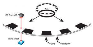
The Channel A output waveform looks like this.
Resolution, when applied to optical encoders, specifies the number of times the output signal goes high per revolution. This number can match the number of lines on a disk; or, especially with higher resolutions, it can be a multiple of the number of lines. (We’ll talk bout this more in the section on Scalability, below.)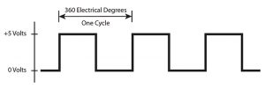
The number of lines on a disk is always related to the resolution. Typical values range from low numbers like 32 or 64 to much higher resolutions of 5,000 or 10,000 and ebyond.
The following picture shows several encoder disks: lower resolutions are on the left and higher resolutions are on the right.
Encoder resolution is measured in units of Cycles Per Revolution (CPR). The word cycle has both a physical and an electrical meaning.
• Physically, on the disk, a cycle is composed of a line/window pair; therefore, in its most basic form, CPR is the same as the number of lines, the number of windows, or the number of line/window pairs.
• Electrically, a cycle refers to one full cycle of the encoder’s output waveform: one high pulse and one low pulse. One cycle is equal to 360° electrical degrees.
CPR, then, can refer to the number of lines and windows on the disk, or the number of electrical cycles in one rotation. Native CPR will be the same number in either case, because each line/window pair is exactly what generates each electrical cycle.
CPR also gives us the smallest distance that can be measured. Divide the total distance of 360° mechanical degrees by the number of cycles per revolution, and the answer will be mechanical degrees per cycle. For example, with an encoder resolution of 3,600 CPR: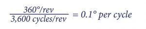
While cycles per revolution is a common term to specify resolution for incremental encoders, some manufacturers use terms like “counts per revolution” (also abbreviated CPR), “pulses per revolution” or “positions per revolution” (both abbreviated PPR), and ther phrases. To avoid confusion, in this paper we’ll use cycles per revolution and CPR.
In the next section, we will use PPR to mean pulses per revolution—but in a different context: resolution multiplication.
Resolution Multiplication
The resolution of a disk is tied to physical reality—physical lines on a physical disk. The number of lines, in its most basic form, is the resolution. However, a motion controller can interpret the output waveforms resulting from those lines and produce higher resolutions— from the same disk.
Incremental encoders commonly use Quadrature. Manufacturers add another LED and photo sensor, displaced from the first LED by 90° electrical degrees. Note that 90° electrical degrees is 1/4 phase or quadrant—which is the origin of the name quadrature.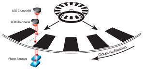
This yields a second output waveform, Channel B, shifted in phase from Channel A by 90 electrical degrees.
Two important results emerge from adding Channel B:
• Direction can now be determined: “A leads B” can indicate clockwise rotation, for example.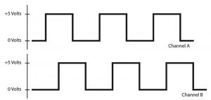
• And more importantly, as related to our discussion – resolution can be multiplied by a factor of 2 or 4
This is called resolution multiplication. System designers can implement it by using an encoder to counter interface chip such as an LS7183N.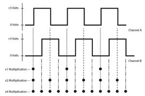
As an example, let’s look at an encoder with 100 lines and windows on its disk. The encoder’s resolution is 100 CPR.
• x 1 – if we count the rising edge of each Channel A pulse as the disk rotates, we’ll get 100 pulses per revolution (100 PPR). This is the same number as the resolution of 100 CPR, as expected for multiplication by 1.
• x 2 – if we count each rising edge and each falling edge of Channel A, we’ll get 2 pulses per cycle, which adds up to 200 pulses per revolution (200 PPR).
• x 4 – if we count each rising edge and falling edge of both Channel A and Channel B, we’ll get 4 pulses per cycle, for a total of 400 pulses per revolution (400 PPR).
Notice we’re not changing the resolution of the disk; it remains set, as determined by the number of cycles per revolution. But by decoding the output waveforms in different ways, we are able get up to 4 times as many pulses per revolution as there are lines on the disk.
Linear Encoders and Resolution
Everything we have said so far about resolution also applies to incremental linear encoders. This makes sense; linear encoders use a linear strip that is equivalent to a circular disk which has been cut along a radius and straightened out. The term Cycles Per Inch (CPI) is used for resolution with linear encoders, although Lines Per Inch (LPI) is also sometimes used.
Absolute Encoders and Resolution
Thus far we’ve discussed incremental optical encoders, whose lines and windows represent relative positions on the disk; each line/window pair looks like every other line/window pair. They are indistinguishable from each other. What matters are the high/low output transitions as each line and window goes past the sensor.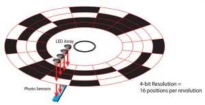
Absolute encoders operate differently. They output a unique code for each position on the disk—each code is absolute, which means that since it is unlike any other code on the disk, it specifies a unique, absolute position on the disk. The next drawing shows a disk for a traditional absolute encoder. It has four tracks, and an LED array with sensors that read the pattern from each track.
Resolution for absolute encoders is defined as the number of positions per revolution as the disk rotates through 360°. Sometimes the equivalent term codes per revolution is used.
You will often see the resolution of an absolute encoder specified in bits. For example, the disk in the drawing above has 4-bit resolution, one bit being produced from each of the four tracks at each position. Higher resolutions would have more tracks; 10-bit resolution would require 10 tracks, for example.
With some designs, each absolute encoder is set at one specific resolution. Some manufacturers, however, take a different approach, and make disks with a single band that contains a unique bar code for each position, as in the next drawing.
An absolute encoder with a bar code can offer programmable resolution: for example, a 12-bit encoder (4,096 positions per resolution) can be programmed to output from 2 to 4,096 codes per revolution.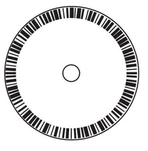
The next table shows how resolution in bits is related to positions per revolution, and degrees of rotation per position.
For a 12-bit absolute encoder, notice that each unique position occupies less than 1/10 of one degree of the disk’s circumference, which is less than 6 arcminutes.
Absolute encoders don’t use quadrature, so there is no equivalent to resolution multiplication that’s available with incremental encoders.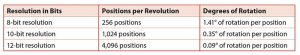
Scalability: Disk Size and Encoder Resolution
Miniaturization is a strong trend in product development. Designers often try to pack more features into increasingly smaller packages. This creates a need for miniature encoders to meet the demand for reduced size. Does reducing encoder size also reduce available resolution? For traditional encoders, the answer was yes.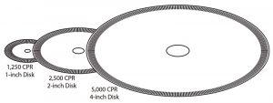
The drawing shows that, for traditional encoders, high resolution requires more lines on an encoder disk. If there’s not enough space for the lines to fit, then the only solution is to make a bigger disk. To double the resolution, you have to double the disk’s diameter.
With newer technology, however, manufacturers can increase the resolution of a disk— without increasing disk size. This is called scalability, and it’s ideal for miniaturization.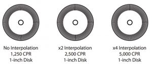
The drawing shows a 1-inch disk with 1,250 lines (1,250 CPR). Through the technique of electronic interpolation (signal processing that takes place within the encoder itself), the CPR can be increased to 2,500 CPR using x2 interpolation; and to 5,000 CPR using x4 interpolation.
In this example, by using interpolation and scalability, we’ve achieved two increasingly higher resolutions—all from the same small encoder disk.
Furthermore, using resolution multiplication (discussed earlier), the 5,000 CPR encoder could be decoded to produce 10,000 Pulses per Revolution (PPR) or 20,000 PPR.
Not all encoder technologies are equally scalable, though:
• Transmissive Optical Encoders: Very scalable
• Reflective Optical Encoders: Very scalable
• Magnetic Encoders: Scalable
• Capacitive Encoders: Not easily scalable
Optical encoders are the most flexible, and best for miniaturization. With capacitive encoders, however, scalability is much more difficult to accomplish; in most cases, to get a higher resolution, you have to buy a larger encoder—if one is even available.
Interpolation is a wonderful way to achieve scalability, but there are limits. At higher and higher resolutions, jitter may become a problem and waveform symmetry can suffer.
If you want higher resolution in a small package, work with your encoder manufacturer. They may be able to provide a custom solution which gives you the resolution you desire, and still avoids signal degradation from jitter or electrical noise.
How Much Resolution Do You Need?
Any particular model of encoder may be available in a range of resolutions. For example, a quick survey of manufacturers might show that a single encoder is available in 20 different resolutions, ranging from 64 CPR to 10,000 CPR.
Is the best practice to always choose the highest resolution? Surprisingly, no. Often it’s better to evaluate your application, and choose the lowest resolution that will satisfy your needs—even if a higher resolution is available.
Here are some reasons higher resolution may not be the best choice:
• COST: higher resolution may cost more.
• PROCESSING TIME: it takes time to read each cycle. Higher CPR = more time.
• HIGH VELOCITY APPLICATIONS: shorter time available to read each cycle.
• JITTER: sensitive systems may over-respond to high resolution information.
• SIZE: In some cases, higher resolutions may have size implications
Resolution and Accuracy: A Preview
When choosing a resolution, a novice designer might look at a specific option in the range of resolutions available, and say, “No; I need more accuracy than that.” What the designer may really mean is, “I need more resolution.”
Resolution and Accuracy: the two terms are often misunderstood and used interchangeably—but they are not the same. What’s the difference? We’ll introduce accuracy in this next section, then revisit the relationship between resolution and accuracy after that.
ACCURACY
Encoders are designed to provide feedback about position, which is used for calculations about angle, distance and velocity. When you command a system to move and then stop at a specific position, you might wonder: is the encoder reporting from the exact target position? Or has it gone beyond, or perhaps stopped short of the target?
Accuracy is the term used to describe the difference between target position and actual position. In an ideal world, they would be the same—but in the real world, there are variations. The actual position—where the encoder really is—might be off from the target position by a small amount, as indicated by the range in the encoder’s accuracy specification.
Measuring encoder accuracy involves a meticulous procedure that requires sophisticated, well calibrated equipment. For example, you can measure a medium-accuracy encoder by using a second, highly accurate “calibration” encoder. If you record target vs. actual for each encoder position through one revolution, then evaluate your results, you can determine the accuracy of the encoder under test. (Will the results be the same if you evaluate the encoder through a second revolution? Or a third? See Precision, below.)
For rotary encoders, accuracy is measured in degrees, arcminutes or arcseconds. Which units are used depends upon the encoder being measured. Degrees might be sufficient for a low accuracy encoder; fractions of a degree or arcminutes are suitable for encoders with medium accuracy; while arcseconds might be used for ultra-high accuracy encoders.
For example, here are specifications for an absolute optical shaft encoder:
![]()
In this case, the encoder’s typical accuracy is 0.18 degrees, which is equal to 10.8 arcminutes.
Below are accuracy specifications from a different manufacturer for another encoder, an optical incremental shaftless model:
![]()
This manufacturer uses the term position error for accuracy, measured in arcminutes. It’s the angular difference between the actual shaft position and the position indicated by the encoder cycle count.
The typical accuracy is similar for both encoders, approximately 0.18 degrees or 10 arcminutes.
Who Controls Accuracy? – Encoder Specifications vs.
System Accuracy
You may consider accuracy specifications for an encoder you’re evaluating, but accuracy doesn’t end there. Encoders are usually part of a larger motion control system. The non-encoder parts of that system can have a dramatic impact on overall system accuracy.
Encoder manufacturers control some of the factors that affect accuracy, while end users control application-specific factors.
Manufacturers
- Placement of pattern on disk: centered or eccentric
- Mounting of hub to disk
- Mounting of disk to shaft (for shafted models of encoder)
- Alignment of optics
End User
- Mounting of encoder disk to motor shaft (for encoder kit
- Mounting of encoder module (for encoder kits)
- Coupling encoder to system (for shafted encoders)
- Stability/rigidity of mounting structure
- Gear tolerances and backlash
- Play in motor bearings
- Axial, radial, side to side, other motions of mechanical parts
- Vibration, temperature, metal fatigue, corrosion, etc.…
It’s easy to see from the partial list above that variations in encoder accuracy may be only a small fraction of the total system accuracy.
How Much Accuracy Do You Need?
As the list above shows, the overall system may be far less accurate than the encoder. In applications with low system accuracy, all that’s required for encoder accuracy may be monotonicity—as the encoder turns, the count constantly increases or constantly decreases.
A monotonic count: …127…128… 129… 130… 131… 132…
A non-monotonic count: …127…128… 129… 128… 132… 131…
A low accuracy encoder can cost less, and as long it provides a reliable, monotonic count, it may be all you need.
As total system accuracy increases, an encoder with medium accuracy might be required. For the majority of applications, encoder accuracy in the range of 0.1° or 8 – 10 arcminutes is sufficient. The two sample encoders discussed above are in this range and are quite affordable.
For applications with extremely close tolerances, high accuracy encoders with specifications in arcseconds are available—but with the increase in accuracy, there will be a corresponding increase in cost.
Resolution and Accuracy: Revisited
Recall the novice designer from the end of the section on resolution, who said, when selecting an encoder resolution, “No; I need more accuracy than that.” We’re now in a position to clear up the very common confusion between resolution and accuracy.
Let’s consider a manufacturer who offers two versions of a magnetic absolute encoder, one with 12-bit resolution and the other with 10-bit resolution.
Starting at zero, here are the first 9 positions, in degrees, that each encoder could report as its disk rotates (some digits omitted for clarity):
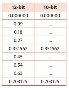
The 12-bit encoder can report 4,096 positions per revolution, which is 4 times as many as the 10-bit encoder’s 1,024 positions. After the 0.0 position, the 12-bit encoder is reporting its fourth reading by the time the 10-bit encoder reports its very first reading.
So which encoder is more accurate? Here is what the manufacturer states in the encoder’s data sheet:
“While the accuracy is the same for both encoders, the 12-bit version provides higher resolution.”
The accuracy is the same. This example shows that accuracy and resolution are not related to each other. One term—accuracy—describes target position vs. actual position. The other term—resolution—describes how finely a disk is divided. These are independent properties.
If our novice designer needs an encoder that can report positions every tenth of a degree, then the designer needs more resolution, not more accuracy—and the 12-bit encoder would be a good choice.
PRECISION
As we saw above in the Accuracy section, to determine the accuracy of an encoder we can rotate the encoder through one revolution of 360° and note the accuracy—the angular difference between target position and actual position—at each encoder count location.
What happens if we go around a second time and measure accuracy again? Do we get the same position error at each location? How about after a third, fourth or fifth rotation? Is the position error repeatable, or does it vary?
Precision is the term that describes repeatability of measurements. It’s the amount that successive measurements differ from each other.
Consider arrows shot by two archers in a competition. Which archer is more accurate?
Surprisingly, the average accuracy is similar for both targets. The average position of all the arrows on the left is in the center of the bullseye, the same as the tight grouping of arrows on the right. The difference between the two lies in the precision of the shots. The group on the left is accurate, but not precise. The group on the right is both accurate and precise.
Now let’s look at arrows shot by two more archers. Which archer is more precise? (see below).
The precision is the same for both archers. The arrows on the left are precise—but they are not accurate. The group on the right is, again, both accurate and precise.
Putting Precision to Work
Precision, then, is the amount that successive measurements differ from each other. An encoder that has position errors which are repeatable may have good precision, even though it may not be perfectly accurate. In this case, the precision can be used to compensate for the inaccuracy of the encoder.
For example, let’s look at successive measurements made for two encoders. The target haft angle is 45.00°.
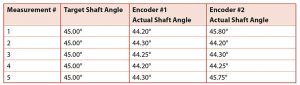
The position error is about 0.75° for each encoder, but while Encoder #2’s errors follow no repeatable pattern, Encoder #1 is more precise—its error is always -0.75°, on average.
Encoder #1’s precision can be put to good use. The error can be tabulated at each position, and those measurements can be used to compensate the encoder’s reported position. For example, adding 0.75° to each of the measurements in the table above will report positions as follows:
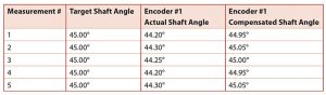
Encoder #1 will now report a compensated position that is within 0.05°of actual position, which is much more accurate than its uncompensated average readings of -0.75°.
In fact, this compensation technique is used when manufacturers produce high accuracy encoders. These encoders are manufactured to standards that ensure that whatever error they have, it’s repeatable. Their precision is used to create a lookup table for error compensation, which is applied to each position the encoder reports.
Precision of an Entire System
The concept of precision applies to every component of a motion control system, not just the encoder. For example, consider a cut-to-length application. An encoder is attached to a motor that drives a ball screw and actuator, which positions wire for cutting.
Suppose the system is set to cut the wire at exactly 12.00 inches. After the first 4 wires are cut, they are measured, with the following results:
11.81 inches
11.82 inches
11.80 inches
11.81 inches
The wires are consistently about 0.20 inches too short. Where is the error coming from? It could be from anywhere—or everywhere—in the system: the encoder itself, the motor, play in the threads of the ball screw or in the bearings of the linear slide.
Because the difference between readings is small, the system has good precision. This can be used to calibrate the application; 0.20 inches can be added to the final target position of 12.00 inches, to end up at a compensated position of 12.20 inches. When the wires are then cut, they will be very close to the desired length of 12.00 inches.
CONCLUSION
We’ve discussed three of the most important concepts related to encoders.
Resolution – the number of cycles per revolution or cycles per inch of an encoder
Accuracy – the difference between target position and actual reported position
Precision – the difference between repeated measurements
While these terms seem interchangeable, they are really independent of each other. Understanding resolution, accuracy and precision will help you make decisions when you choose an encoder.
About US Digital:
With over a million off-the-shelf configurations, plus any number of custom product offerings, US Digital® has delivered quality in motion since 1980. US Digital offers stellar service, delivering motion control solutions best suited to each unique need. Automated systems, continuous improvement protocols and stringent testing ensures we bring quality to every product manufactured.
Located in Vancouver, Washington, the vertically integrated facility and stellar service team provides customers with exceptionally short lead-times, offering same-day fulfillment on most orders.
Visit usdigital.com or contact: info@usdigital.com